Health-Related Quality of Life Modeling of Adolescent & Young (AYA) Adult Cancer Patients

A tri-layer hybrid simulation of health-related quality of life (HRQoL) from diagnosis through survivorship in adolescent and young adult (AYA) cancer patients, ages 15–39, coupling an agent-based model of patients, an evolving social-support network, and a system-dynamics model of population and services.

Principal Investigator: Joseph Blochberger, MSME, PE. Active PhD research with a methodological focus. Currently seeking collaborators across Johns Hopkins Medicine, Public Health, Nursing, and Social Work.

Agent-Based ModelingNetwork Modeling and Analysis System DynamicsHybrid Modeling MATLAB, reproducibleOpen to Collaboration AYA CancerQuality of Life

Abstract

Background. Health-related quality of life (HRQoL) in adolescent and young adult (AYA) cancer patients is worse than population norms, with the largest deficits in physical and emotional functioning, and persists for years after diagnosis[1, 2] Clinical and observational studies capture HRQoL at limited time points and cannot represent the joint, evolving influence of patient heterogeneity, social support, and service-system feedback.

Methods. A tri-layer hybrid simulation model couples an agent-based model of individual patients, an evolving social-support network, and a system-dynamics model of population and services. The three layers exchange information through six explicit interfaces, each of which can be disabled independently to measure the contribution of each interface. No prior model is known to couple all three layers for AYA HRQoL[16, 17]

Results. Over 20 simulation seeds and a 24-month horizon, the model reproduces patterns it was not fitted to, including a treatment nadir, persistent emotional deficits, and a durable-remission fraction near 78% among treated agents, within the band anchored to AYA 5-year relative survival[1, 5] Each interface acts in the direction predicted by the governing mechanism, with effect sizes that differ sharply: social support dominates the outcome while the population-feedback loop is near-dormant under baseline parameters. All interface verification checks pass, including a no-leak test, a structural verification method used to ensure that stocks (accumulations) do not gain or lose material spontaneously. It checks that all inflows and outflows are properly accounted for and that no hidden or "leaking" flows exist[9]

Conclusions. The model stands as an exploratory scaffold for theory and decision support. Predictive validation against a longitudinal AYA cohort remains open. OPEN

Model card

Purpose, anchoring evidence, and stated limitations, each expanded in the sections that follow.

PurposeTheory development and decision-support scaffold for AYA HRQoL trajectories and candidate interventions, for example NCCN distress screening and financial navigation.
Intended usersResearchers and clinician-scientists in AYA oncology, survivorship, and health-systems modeling.
Not forIndividual prognosis or clinical decisions for a specific patient.
PopulationAYA cancer patients, ages 15–39, diagnosis through about 24 months (extensible).
Empirical anchorsAYA HOPE,[1] SURVAYA,[3] SEER survival,[5] EORTC QLQ-C30[15] reference values,[4] and pooled intervention effect sizes including nulls.
Key limitationsPredictive validation open; long-term heterogeneity under-dispersed; several parameters flagged for provenance; the population-feedback layer is near-dormant under baseline parameters and activates only under stress; single network, with the psychometric/social distinction left to future work.
ReproducibilityMATLAB R2024b, no toolboxes; fixed seeds; one-command figure regeneration.
StatusVerified prototype; iterative validation in progress.

Background

Understanding how HRQoL evolves after an AYA cancer diagnosis is essential to improving survivorship care. Three findings define the burden this work addresses:

Clinical and observational studies capture HRQoL at limited time points and cannot represent these factors as they interact and evolve. Simulation can. Most simulation work, however, couples only one or two paradigms; the difficulty, and the contribution here, is the interfaces between three. This work develops a tri-layer hybrid model and tests whether each layer earns inclusion.

Scope

This model explores which mechanisms and interventions plausibly shape AYA HRQoL; it does not predict outcomes for an individual patient. Predictive validation remains open.

Empirical basis: incidence, age, and diagnosis

The model targets the adolescent and young adult (AYA) population and distinguishes outcomes by diagnosis. The first three figures give the empirical basis from published evidence. The fourth is a model output: cancer type enters the verified simulation only through cited inputs (5-year survival and treatment intensity), and HRQoL emerges by diagnosis. Inputs taken from the project AYA dataset are literature-informed estimates flagged for provenance verification, so these figures are exploratory; comparisons across pediatric and older-adult groups stay empirical, since the simulation spans ages 15-39.
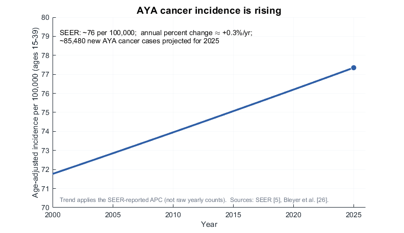
AYA cancer incidence rising over time
AYA cancer incidence is rising. Age-adjusted incidence in ages 15-39 trends upward at the SEER-reported annual percent change[5, 26]
  • AYA (15-39) age-adjusted incidence is about 76 per 100,000 and rising at roughly +0.3% per year
  • About 85,480 new AYA cancer cases are projected for 2025
  • The upward trend motivates a population-level, longitudinal modeling focus on AYA survivorship
  • The plotted line applies the published annual percent change and does not show raw year-by-year counts
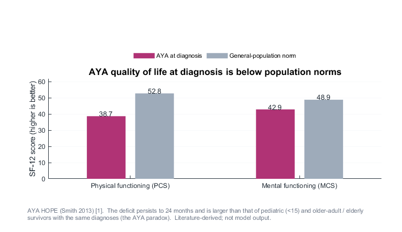
AYA HRQoL below population norms
AYA HRQoL is below population norms. SF-12 physical and mental scores at diagnosis sit well under the general-population norm[1]
  • At diagnosis, AYA physical (PCS 38.7) and mental (MCS 42.9) scores fall far below the norms (52.8 / 48.9)[1]
  • The deficit persists to 24 months rather than resolving after treatment[2]
  • AYAs score lower than pediatric and older-adult survivors with the same diagnoses (the AYA paradox)
  • The below-norm pattern holds across diagnoses, which is the empirical case for an AYA-specific model
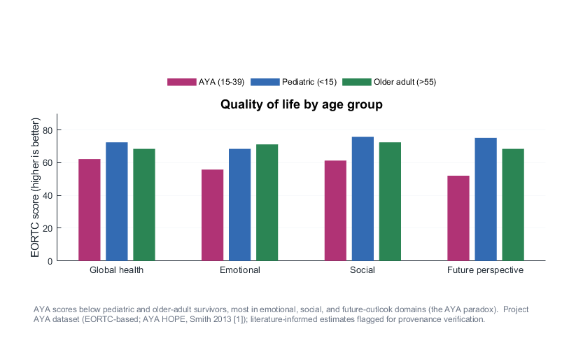
HRQoL by age group
HRQoL is lowest in AYA across age groups. EORTC-domain scores for AYA, pediatric, and older-adult survivors[1]
  • AYA survivors score below both pediatric and older-adult survivors on every domain shown
  • The gap is largest for emotional functioning and future perspective, the AYA-specific domains
  • Older adults score near or above pediatric on emotional and social, which isolates the AYA dip
  • Values are the project AYA dataset (EORTC-based; AYA HOPE [1]), flagged for provenance verification
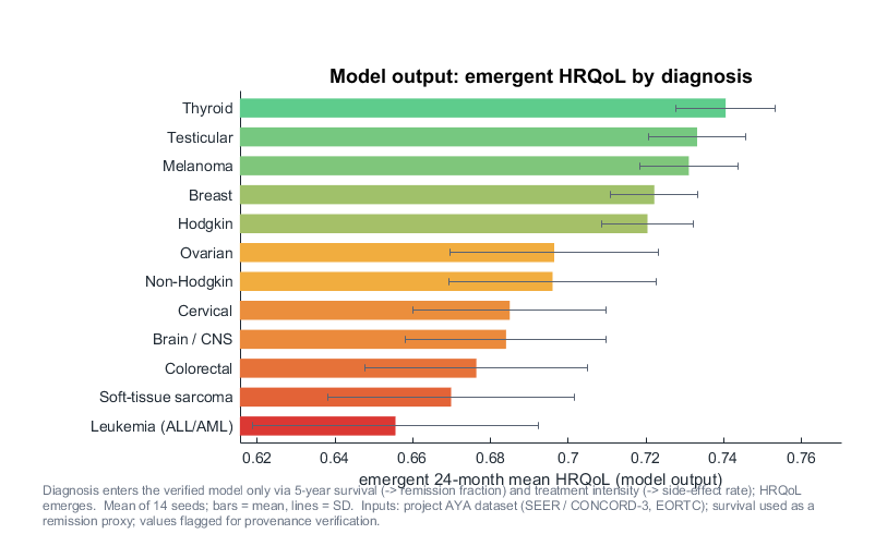
Model HRQoL by diagnosis
Model output: HRQoL emerges by diagnosis. Cancer type enters the verified model only through 5-year survival and treatment intensity. The 24-month HRQoL emerges from those inputs rather than from a fitted target[5, 30]
  • High-survival, lower-intensity cancers (thyroid, testicular, melanoma) reach the highest HRQoL
  • Low-survival or intensive-treatment cancers (leukemia, colorectal, sarcoma) reach the lowest
  • The ordering emerges directly from the cited inputs, survival and treatment
  • Inputs are flagged estimates and survival stands in for durable remission, so the figure supports exploration rather than forecasting

Methods: three autonomous layers, six interfaces

The model comprises three layers, each with a separate state and separate update rules. The layers exchange information through six explicit interfaces, and each interface can be disabled independently, which allows the contribution of each one to be measured.

Conceptual framing: how this differs from the usual hybrid

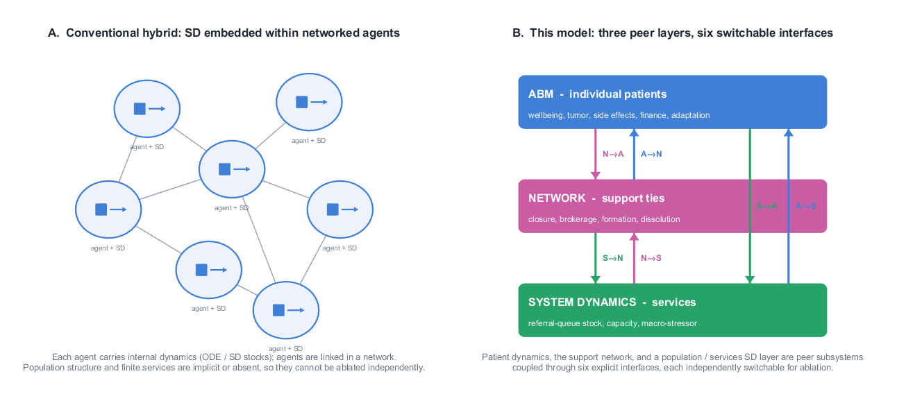
Hybrid simulation most often nests system dynamics inside agents: each agent carries an internal set of continuous dynamics, and the agents interact, often over a network. Population structure and finite shared services are then implicit in the aggregate of agent states. This model retains per-agent dynamics but also promotes the support network and a finite-capacity services subsystem to peer layers, coupled through six explicit, switchable interfaces, so the contribution of each can be isolated and measured. A fuller treatment is in docs/CONCEPTUAL_FRAMING.md.

Conventional SD-in-agents hybrid versus the three peer layers of this model
Conventional hybrid (A) versus this model (B). Conventional hybrid designs nest system dynamics inside networked agents and leave population or service structure implicit. This model instead runs patient dynamics, the support network, and a system-dynamics services layer as peer subsystems, coupled through six independently switchable interfaces.
  • System dynamics, networks, and agents are each established individually; the novelty is the verified, switchable coupling of all three as peer layers
  • Elevating finite services to a peer layer is what lets the population-feedback effect be isolated, switched off, and measured
  • The per-agent wellbeing core is itself a small SD system, so the model both embeds dynamics in agents and couples them to an aggregate services layer
SW_NA: support → psychological buffer SW_AN: withdrawal → ties dissolve SW_AS: distress → referral demand SW_SA: stress / access → psychological SW_SN: program capacity → ties form SW_NS: ties → referral diffusion ABM individual patients NETWORK evolving social ties SYSTEM DYNAMICS population & services
All six interfaces are implemented and pass verification, including a no-leak test confirming that a disabled interface transfers nothing[9]

What each layer owns

LayerState it ownsAutonomy
ABM (patients)physical and psychological wellbeing, tumor burden, side effects, financial toxicity, adaptationruns standalone
Network (ties)who supports whom; ties form and dissolve over time evolves under independent rules
System dynamicsreferral-queue stock, service capacity, population stress integrates genuine stock-flow state

Feedback structure (causal loop diagram)

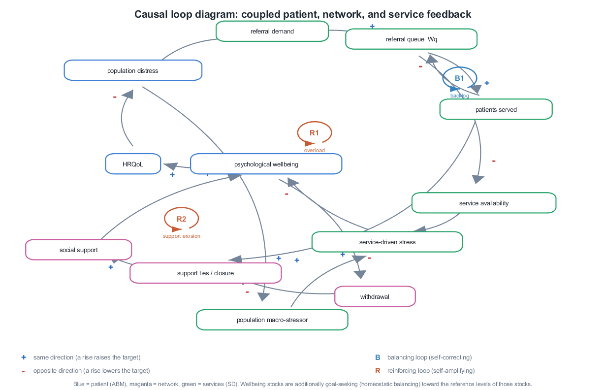
The feedback structure is the essential part of the coupling. The causal loop diagram below renders it in the convention used by system-dynamics articles: named variables, causal links carrying a plus or minus polarity, and labeled balancing (B) and reinforcing (R) loops. A stock-and-flow view of the services layer is in the diagrams section, and a guide to constructing such interfaces is in docs/CONSTRUCTING_INTERFACES.md.

Causal loop diagram of the coupled patient, network, and service feedback
Causal loop diagram of the coupled feedback. Plus and minus signs give the polarity of each causal link; B and R mark balancing and reinforcing loops.
  • B1 (backlog). Serving patients drains the referral queue, a self-correcting balancing loop
  • R1 (overload). A full queue lowers service availability, which raises stress and distress, which raises demand, which fills the queue further: a reinforcing loop that is latent at baseline and activates under stress
  • R2 (support erosion). Falling wellbeing raises withdrawal, which dissolves ties and lowers support, which lowers wellbeing further: the social vicious or virtuous cycle
  • Wellbeing stocks are also goal-seeking (homeostatic balancing) toward the reference levels of those stocks, which is what produces the recovery after the treatment nadir

Network model and node definition

What the nodes are

Each node is an AYA patient-agent, the same agents as the ABM layer; an edge is a peer support tie between two patients. Support reaches a patient through the single N→A operator, built from two literature-grounded parts. The first is structural emotional support set by network closure: the local clustering coefficient of a patient sets how much emotional and esteem support that position affords, since closure (densely interconnected contacts) predicts emotional and esteem support, while brokerage predicts informational support[59, 60, 61] The term is weighted by tie strength, since strong, multiplex ties carry emotional aid,[62] and saturates with connectedness, the diminishing returns implied by the dose-response between network size and outcomes[6] The second, smaller part is complex-contagion reinforcement: wellbeing lifts only when several neighbors are thriving, so the effect travels along clustered, wide-bridge ties rather than single shortcuts, the form social reinforcement takes for behavioral and psychosocial spread[58, 63] Referral diffusion runs the opposite direction through brokerage: the N→S interface routes help-seeking along non-redundant broker ties, since brokerage carries informational support while closure carries emotional support[59, 60] An isolated patient (degree zero) carries a small penalty.

The simplification is deliberate. Real AYA support systems are heterogeneous and ego-centric, but small: a typical support network holds roughly 2 to 10 members (mean about 6), about 40% family and 60% non-family, alongside 3 to 5 clinicians[70, 6, 20] Each run draws a network size from this distribution (mean 6, SD 2.2, range 2 to 10), so the simulated cohort spans sparsely to well connected patients rather than sharing one fixed degree. The current model collapses family, peer, clinician, navigator, and digital ties into one homogeneous patient-peer tie type. Peer structure is the AYA-distinct, intervention-relevant channel, through peer-mentoring programs,[21] so it is modeled first; a typed support network is identified as future work.

Why a small-world (Watts-Strogatz) network

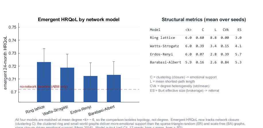
The default initial topology is a Watts-Strogatz small-world graph[55] Real social networks combine high local clustering with short global path lengths, the small-world signature, which neither a regular lattice (clustered but distant) nor an Erdos-Renyi random graph (short but unclustered) reproduces[57] Because emotional support here is driven by network closure and the wellbeing-contagion term is a complex, reinforcement contagion, both of which reward clustering, the choice of topology now changes the outcome[59, 63] Both mechanisms favor more clustering, so the ring lattice, the most clustered graph, scores highest. The small-world topology is used regardless, because it matches the realistic structure of human social networks, high clustering with short paths[55] The comparison below holds mean degree constant across topologies to isolate the effect of network structure.

Degree-matched network-model comparison
Degree-matched comparison of network models. Four initial topologies at mean degree near 6, injected into the full model; emergent HRQoL with structural metrics alongside[55, 56, 57]
  • The structural metrics recover the textbook signatures; the small-world graph keeps high clustering (C = 0.39) with a short path length (L = 3.4), while the random graph has near-zero clustering (C = 0.07)
  • Emergent HRQoL tracks clustering: ring (C = 0.60) reaches 0.723, small-world (0.39) 0.719, scale-free (0.16) 0.713, and random (0.07) 0.712, so the outcome is sensitive to which topology is chosen
  • Closure carries emotional support[59] and complex contagion travels on wide bridges;[63] both reward clustering, which is why clustered topologies deliver more support
  • Every topology still lifts HRQoL above the no-network baseline; closure adds a further, ordered increment on top of that social-structure contribution

Extension: a typed support network EXPLORATORY

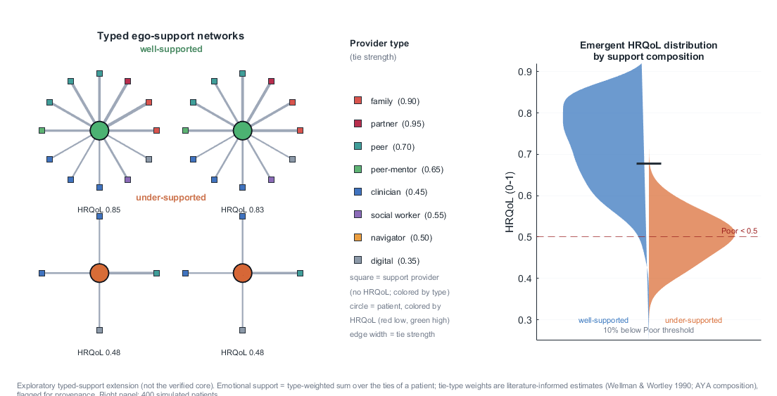
The verified model uses one homogeneous patient-peer tie. A typed-support extension replaces it with an ego-network of providers for which tie strength and support profile are set by relationship type: family and partners are the strongest emotional sources for AYAs, clinicians carry informational support, and social workers and navigators carry instrumental support[59, 62] Provider nodes have no HRQoL and are colored by type; patients are colored by HRQoL. The tie-type weights are literature-informed estimates flagged for provenance, so this extension is exploratory and is not part of the calibrated core.

Typed support network with providers colored by relationship type
Tie strength grounded in relationship type. Sample typed ego-networks (left) with a provider-type legend (center) and the population HRQoL distribution that emerges when emotional support is the type-weighted sum over the ties of a patient (right).
  • Tie strength now depends on relationship type rather than a single random weight: family (0.90) and partner (0.95) ties carry the most emotional support, clinician ties (0.45) the least
  • Well-supported patients (more family, partner, and peer ties) reach HRQoL near 0.85; under-supported patients (few emotional ties, mostly clinicians) fall to about 0.48
  • Across a simulated population, support composition alone produces a wide HRQoL distribution with about 10% below the Poor threshold, concentrated among under-supported patients
  • Typed ties point to a concrete next step for intervention design: target the specific support type a patient lacks, instead of adding undifferentiated connections

Data sources feeding the model

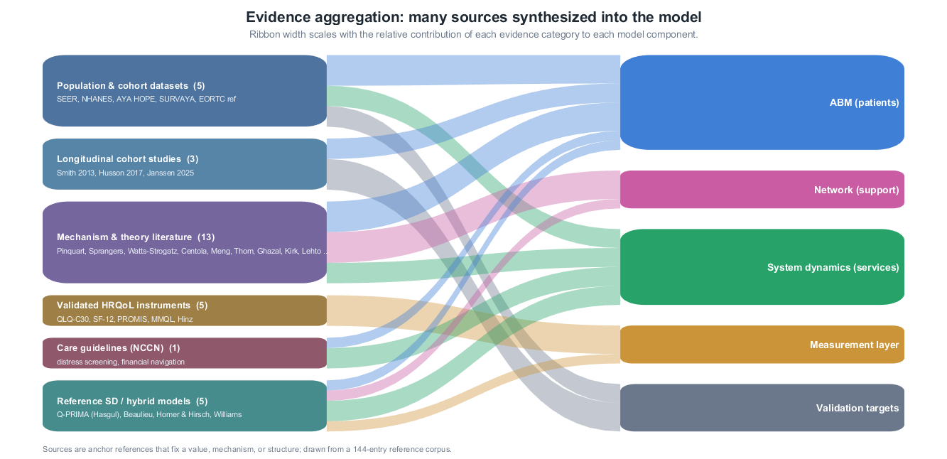
Model parameters, the observation layer, and the validation targets are anchored to published evidence and public datasets. The diagram below traces each source to the model component it informs, the table lists what each one contributes, and full citations appear in the references section.

SEER: AYA incidence, 5-yr survival (~86%) 5-year relative survival [5] AYA HOPE (Smith 2013) + NHANES baseline HRQoL & depression [1] [54] Social support (Pinquart); response shift (Sprangers, Bellizzi) [6] [10] [11] NCCN AYA guidelines screening, financial navigation [30] EORTC QLQ-C30 + reference values PROMIS, MMQL instruments [15] [4] [29] SURVAYA (Janssen), Husson 2017 long-term HRQoL targets [3] [2] ABM individual patients NETWORK evolving support ties SYSTEM DYNAMICS population & services MEASUREMENT LAYER instrument scales VALIDATION TARGETS held-out bands
Source evidence (left) feeds the agent, network, and system-dynamics layers, the measurement layer, and the held-out validation targets (right).

How the evidence was aggregated

Six categories of evidence, spanning public datasets, longitudinal cohort studies, mechanism and theory literature, validated instruments, care guidelines, and reference models, feed the model components they inform. The map below shows the relative contribution of each category. The breakdown that follows adds the provenance-tier composition, the source counts, and a worked example of how several sources reconcile into model terms.

Evidence aggregation map: source categories flowing into model components
Evidence aggregation map. Six evidence categories (left, with source counts) feed the five model components (right). Ribbon width scales with the relative contribution of each category to each component.
  • Mechanism and theory literature is the broadest input, informing the patient, network, and service layers
  • Datasets and cohort studies anchor patient initialization and the held-out validation targets
  • Instruments feed the measurement layer; reference models (including Q-PRIMA) inform structure across all layers
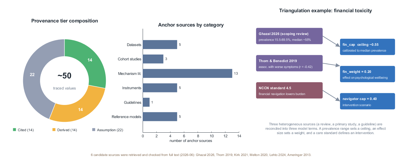
Provenance tier composition, source-category counts, and a triangulation example
Provenance breakdown. Tier composition of the roughly fifty traced parameter values, the number of anchor sources per category, and a triangulation example for financial toxicity.
  • About 28% of values are Cited, 28% Derived, and 44% disclosed assumptions, each justified in writing
  • Triangulation example: a prevalence range, an effect size, and a care standard from three separate sources are reconciled into three model terms
  • Six candidate sources were retrieved and checked from full text (author, year, and value confirmed) in the 2026-06 cycle
Data sourceWhat it providesFeedsRef.
SEER (NCI)AYA incidence; 5-year relative survival (~86%)ABM remission; SD population[5]
AYA HOPE (Smith 2013)Baseline HRQoL; ~20% vulnerable subgroup at diagnosisABM initialization[1]
NHANES (CDC)AYA depression prevalenceABM psychological baseline[54]
Social-network meta-analysis (Pinquart & Duberstein)Direction and magnitude of the social-support effectNetwork to patient (N→A)[6]
Response-shift theory (Sprangers; Bellizzi)Adaptation / recalibration mechanismABM adaptation[10][11]
EORTC QLQ-C30 (Aaronson) + reference values (Hinz)Instrument scales; normative valuesMeasurement layer[15][4]
PROMIS (Siembida); MMQL (Bhatia; Goodman)AYA-validated HRQoL instrumentsMeasurement layer[29][27][28]
SURVAYA (Janssen); HussonLong-term and 24-month HRQoL distributionsValidation targets[3][2]
NCCN AYA guidelinesDistress-screening and financial-navigation care processesSD scenarios[30]
AYA HRQoL review (Sodergren); SD-in-cancer precedents (Williams; Homer & Hirsch)Parameter ranges; design precedentModel structure[20][37][32]
Reference models: Q-PRIMA (Hasgul); CLD (Beaulieu)Structure and docking comparisonWhole model[16][17]

Parameter provenance

Beyond the data sources above, every model parameter and embedded constant is traced to a data source, a paper, or an explicit assumption in the provenance register (docs/PARAMETER_PROVENANCE.md); the model code carries inline [Cited] / [Derived] / [Assumption] tags that point to it. Values fall into three tiers.

TierMeaningApprox. countExamples
CitedValue or narrow range taken from a data source or paper~14 AYA age 15–39 [SEER]; 20% vulnerable subgroup [Smith 2013]; ~86% 5-year survival [SEER]; complex-contagion threshold ≥2 [Centola & Macy 2007]; closure to emotional support [Meng 2016]
DerivedCalibration value for which the mechanism or range is cited~14 financial-toxicity ceiling at ~55% prevalence [65] and the effect on wellbeing [64]; distress threshold within 19.6–61.6% prevalence [66]; tie formation as networks expand after diagnosis [68]; symptom trajectory [69]; service capacity [67]
AssumptionStructural, computational, or calibration choice with no direct empirical anchor~22 tumor kinetics; the wellbeing-equation coefficients; beta_social; alpha_macro; equal weighting of physical and psychological HRQoL

The full parameter table, the stock / flow / auxiliary equation listing, and a written justification for every assumption are in the Parameters & equations section below.

About half of the values are calibration or structural assumptions, and several are swept in the sensitivity and stress experiments. The Derived sources were retrieved and checked (author, year, and the cited value or finding confirmed). One parameter is flagged as weakest-supported: the tie-dissolution rate rests on qualitative withdrawal reports,[31] whereas the strongest longitudinal evidence finds networks net-expand after diagnosis,[68] a pattern the model in fact reproduces. The equal-weight composite is a known simplification relative to the regression-weighted SF-12 summary scores.

Parameters & equations

The model is specified in the stock / flow / auxiliary form used by published system-dynamics models, so the structure can be read and audited directly. The temporal design is diagnosis-anchored (the clock starts at diagnosis) over a 24-month horizon, with fast patient dynamics integrated every half day and the service queue and network restructuring resolved monthly. Every parameter traces to a source or a flagged assumption, and each assumption carries a written justification. A workbook in a four-sheet layout available: AYA_parameters_and_equations.xlsx.

Run specifications

SettingValueUnitNote
Initial time0dayAnchored at diagnosis / cohort enrollment
Final time730day24-month horizon
Time step (patient layer)0.5dayExplicit Euler step for the agent-based layer
Structural cadence30dayMonthly service queue and network restructuring
Treatment window30 to 120dayActive-treatment block; nadir near month 4
Population100agentsInference at the run level, not the agent

How the timeline compares with other SD models

The diagnosis-anchored, population-level, hybrid design departs deliberately from an event-anchored single-patient pure-SD model such as Q-PRIMA (Hasgul 2024)[16] Full discussion and the complete equation listing are in docs/MODEL_TIMELINE_AND_EQUATIONS.md.

DimensionThis modelQ-PRIMA (Hasgul 2024)
ParadigmHybrid: ABM + network + SDPure system dynamics
Time anchorDiagnosis (t = 0)Infusion event (t = 0)
Time span0 to +730 days (24 months)−60 to +180 days (~8 months)
Unit of analysis100 heterogeneous agents1 representative patient
Stocks1 service stock + per-agent states + network14 continuous stocks
Feedback6 switchable cross-layer interfaces7 reinforcing + 2 balancing loops

State variables (stocks)

ABM patient layer NET network layer SD services layer

LayerStockUnitsIntegral form
ABMPhysical wellbeing PDmnl [0.2,1]∫ (P adjustment) dt + P(0)
ABMPsychological wellbeing ΨDmnl [0.2,1]∫ (Ψ adjustment) dt + Ψ(0)
ABMTumor burdenDmnl [0.001,1]∫ (growth − removal) dt + Tumor(0)
ABMSide-effect severity SEDmnl [0,1]∫ (development − removal) dt
ABMFinancial toxicity FinDmnl [0,1]∫ (accrual) dt
ABMAdaptation AdaptDmnl [0,1]∫ (adaptation rate) dt
NETSupport ties A ijDmnl {0,1}formation − dissolution (monthly)
NETTie weights W ijDmnl [0,1]assigned on formation
SDReferral queue Wqpersons∫ (demand − served) dt

Derived (not integrated): HRQoL Q = (P + Ψ)/2; closure Ci (recomputed monthly); in_remission (a latch).

Flows (rates)

LayerFlowCadenceEquation
ABMtumor growth0.5 dg · Tumor · (1 − Tumor)
ABMtumor removal0.5 dtreated: tx_resp · Tumor; remission: remission_decay · Tumor
ABMSE development0.5 din treatment: se_dev_rate · (1 − SE)
ABMSE removal0.5 dse_rem_rate · SE
ABMfinancial accrual0.5 dfin_accrual · [day > tx_start] · (fin_cap − Fin)
ABMadaptation rate0.5 dadapt_rate · (1 − Adapt)
ABMP adjustment0.5 d(target_P − P) / adjustT
ABMΨ adjustment0.5 d(target_Ψ − Ψ) / 21
SDreferral demand (inflow)30 dsee auxiliaries (SW_AS, SW_NS)
SDserved (outflow)30 dmin(Wq, Cpsy)
NETtie formation30 dround(formation_rate · served) (SW_SN)
NETtie dissolution30 dprob = dissolve_rate · 0.5 · (withdrawal_i + withdrawal_j) (SW_AN)
Auxiliaries and the six interfaces (show 16)
Layer / interfaceAuxiliaryEquation
ABMHRQoL Q(P + Ψ) / 2
ABMtarget_Pclip(0.90 − 0.5·Tumor − 0.4·SE + ben_phys, 0, 1)
ABMtarget_Ψclip(0.75 + support + ben_psy − stress − 0.30·SE − eff_chronic, 0, 1)
ABMeff_chronic(identity_pen + fertility_pen + fin_weight·Fin) · (1 − adapt_efficacy·Adapt)
NET N→Astructural supportbeta_social · closure_gain · conn
NET N→Aconnectedness conn1 − exp(−strength / support_scale)
NET N→Aclosure gain(1 − closure_share) + closure_share · (Ci / clustering_ref)
NET N→Acontagionbeta_social · cont_w · logistic((n_supp − 2)/reinforce_width)
SD S→Aservice-mediated stressmacro_stressor · (1 − min(1, service_avail))
SDmacro stressoralpha_macro · max(0, poor_prev − 0.1)
ABM A→Sself-referral demandsum_i [Q_i < distress_threshold] · self_referral_rate
NET N→Sbrokerage ES (Burt)deg − 2·tri / max(deg, 1)
NET N→Sbrokered demandsum_i distressed_i · (0.5 + 0.5·reach_i)
SDservice availabilityserved / max(demand, 1)
ABM A→Nwithdrawalmax(0, withdraw_thresh − Ψ)
SD S→Nserved → tie formationround(formation_rate · served)

The six switchable interfaces are the cross-layer auxiliaries in bold: N→A support, S→A stress, A→S demand, N→S brokerage, S→N formation, A→N dissolution. Setting a switch to 0 removes exactly one of these, which is the basis of the ablation ladder.

Parameters and provenance

Cited value or narrow range from a source Derived mechanism/range cited, value calibrated Assumption no direct anchor; each value carries a written justification

ParameterValueTierSource / basis
age_range[15, 39]CitedStandard AYA definition (SEER / NCI)
T (horizon)730 dDerived24-month follow-up (Smith 2013; Husson 2017)
vulnerable fraction0.20CitedLowest baseline HRQoL quartile (Smith 2013)
responder_fraction0.86CitedSEER AYA 5-year relative survival ~86%
intervention_effect0.13CitedPooled AYA psychosocial intervention SMD
k_neighbors2–10 (mean 6)CitedAYA support-network size, drawn per run (Cloyes 2022)
p_rewire0.15CitedSmall-world regime (Watts & Strogatz 1998)
reinforce_count2CitedComplex contagion ≥2 contacts (Centola & Macy 2007)
adapt_efficacy0.60DerivedA-priori from benefit-finding theory; swept (Bellizzi 2012)
closure_share0.5DerivedClosure predicts emotional support (Meng 2016)
formation_rate0.5DerivedNetworks expand after diagnosis (Lehto 2024)
fin_weight0.20DerivedFinancial toxicity worsens symptoms (Thom & Benedict 2019)
distress_threshold0.5DerivedDistress prevalence band (Kirk 2021; NCCN)
psy_capacity (Cpsy)8 / moDerivedFinite, variable psycho-oncology staffing (Melton 2020)
Q = (P+Ψ)/2equal weightAssumptionSame HRQoL definition as Q-PRIMA; flagged simplification
tumor_growth_base0.045AssumptionLogistic form as in Q-PRIMA; rate calibrated
beta_social0.04AssumptionDose-response (Pinquart 2010); calibrated to ablation; swept
alpha_macro0.4AssumptionLatent-amplifier gain; swept in stress scenarios

Full table (~50 values) and the inline prov: code tags are in docs/PARAMETER_PROVENANCE.md.

Assumption justifications

An assumption marks a value with no source for the exact number. Each one is justified in writing and classified by the type of support behind it. Several wellbeing-core choices inherit structure directly from the published Q-PRIMA model[16]

Justification for every assumption-tier parameter (show 15)
ParameterCategoryBasis
dt = 0.5 dNumerical / Model precedentExplicit Euler, as in Q-PRIMA; step well below the fastest time constant
N = 100ComputationalMonte Carlo sample; inference at run level, seed-averaged
treated_fraction = 0.85Literature mechanismMost AYA cancers treated with curative intent; value illustrative
tx_start/tx_durationPattern-oriented~3-month block placed so the nadir lands near month 4 (Husson 2017)
tumor_growth_base = 0.045Model precedent / Pattern-orientedLogistic form as in Q-PRIMA; rate calibrated with tx_resp
tx_resp = 0.06Pattern-orientedSet with responder_fraction 0.86 so ~86% reach remission
Q = (P+Ψ)/2Model precedentIdentical HRQoL definition published in Q-PRIMA; equal weighting flagged
target-seeking forms, 21-d lagModel precedent / Lit. mechanismHomeostatic restoring (gap / adjustment time) as in Q-PRIMA
target_P, target_Ψ coeffsPattern-oriented / Lit. mechanismCalibrated to SF-12 PCS/MCS anchors; emotional deficit (Smith 2013)
fin_accrual = 0.02Lit. mechanism / Pattern-orientedFinancial toxicity accrues over treatment (Thom 2019)
beta_social = 0.04Lit. mechanism / SweptSupport dose-response (Pinquart 2010); calibrated to ablation; swept
W tie weightsFlagged limitationRandom placeholder; should be type-based (Wellman & Wortley 1990)
withdraw_thresh = 0.55Pattern-orientedJust above the 0.5 distress threshold
alpha_macro = 0.4Swept / Pattern-orientedLatent amplifier; swept in stress scenarios
poor-fraction trigger = 0.1Literature mechanism10% floor below cancer distress prevalence 20–50% (Kirk 2021)

Pattern-oriented means a value is not free but jointly constrained with others to reproduce several observed patterns at once (baseline distribution, nadir timing, recovery plateau, persistent tail), the standard defense in pattern-oriented modeling[7] Swept parameters carry a further protection: the conclusions hold across a range of values rather than resting on one tuned number. Full write-up: docs/ASSUMPTION_JUSTIFICATIONS.md.

Model implementation

The model is implemented in plain MATLAB (R2024b, no toolboxes). Four excerpts show the design decisions that keep the layers separable and the validation sound.

1. Each interface is a binary switch, so the ablation experiment can turn any one of them off in isolation (coupling_switches.m).

% {name, abm_on, AS, SA, AN, NA, SN, NS, description}
'C1',  true, 0,0,0,0,0,0, 'ABM-only (heterogeneity baseline)'
'C3',  true, 0,0,1,1,0,0, 'ABM + Network'
'C4',  true, 1,1,1,1,1,1, 'Full model (all six interfaces on)'

2. Social support reaches a patient through exactly one channel, so disabling that channel removes the effect completely (AYA_MVP_Coupled.m).

% N->A : social support (THE ONLY support channel; no leak)
support = zeros(N,1);
if sw.SW_NA
    deg = sum(A,2);  WA = A .* W;
    support = baseline_sup + contagion + buffer;   % connection, contagion, buffering
    support(deg==0) = -0.01;                        % isolation penalty
end

3. System dynamics holds a real integrated stock, a referral queue, rather than a simple count of agents in a category.

Wq = Wq + demand;                       % inflow: referrals from distressed agents
served = min(Wq, Cpsy);                  % outflow bounded by service capacity
Wq = max(0, Wq - served);
service_avail = served / max(demand,1); % feeds back to patients via SW_SA

4. Verification: turning a coupling off must change the outcome, proving no hidden proxy leaks (verify_interfaces.m)[9]

cOff = cOn;  cOff.SW_NA = false;
v9 = (run_mean(cOn,1:15) - run_mean(cOff,1:15)) > 1e-3;   % PASS = separable

Model diagrams

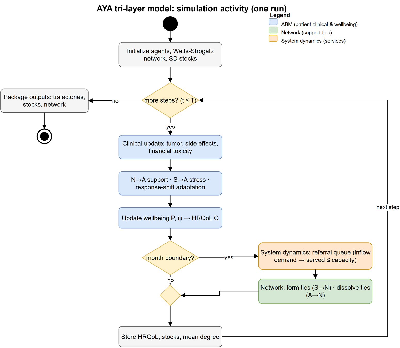
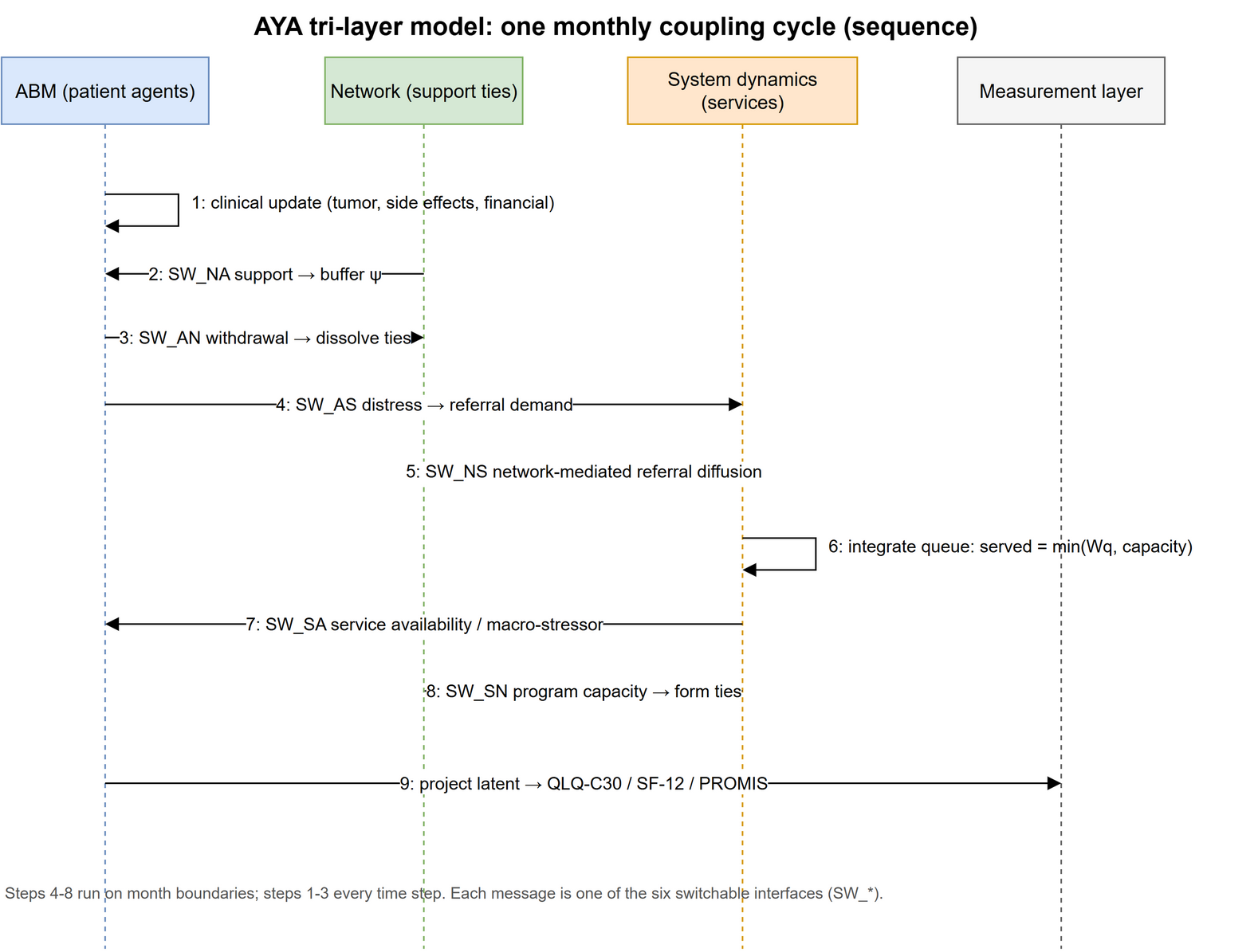
Three UML views document the implementation at the level a reader needs to reproduce or audit it: an activity diagram for control flow within one run, a sequence diagram for the order in which the six interfaces fire over a monthly cycle, and a component diagram for the static structure of the code. A fourth view, a stock-and-flow diagram, documents the internal mechanics of the system-dynamics layer. All are rendered from editable sources in website/diagrams/ (provided as both .drawio and .xml) and use a fixed layer color key: blue for the ABM (patient) layer, green for the network (support) layer, and orange for the system-dynamics (services) layer.

Activity diagram of one simulation run
Activity diagram: control flow of one run. A single run initializes the agents, the Watts-Strogatz support network,[55] and the system-dynamics stocks, then loops over time steps. Patient-layer updates run every step; the system-dynamics queue and network rewiring resolve on month boundaries before the loop stores outputs and advances.
  • Patient clinical and wellbeing updates run every time step; service and network updates resolve only on month boundaries, which fixes the order of operations within a step
  • The month-boundary branch is where the system-dynamics referral queue and network tie formation and dissolution enter, keeping slow population processes separate from fast individual ones
  • HRQoL Q is computed from wellbeing and the support buffer inside the loop, so the trajectory emerges from the simulation instead of following a scripted curve
  • One exit packages trajectories, stocks, and the network, which matches the single output structure the figure and animation scripts read
  • A box-by-box walkthrough of every activity (what it does, the cadence, and the equation it maps to) is in docs/ACTIVITY_DIAGRAM_WALKTHROUGH.md
  • Editable source: model_activity.drawio / .xml
Sequence diagram of one monthly coupling cycle
Sequence diagram: one monthly coupling cycle. Four lifelines (ABM, network, system dynamics, measurement) exchange nine messages. Each cross-lifeline message is one of the six switchable interfaces, so disabling a switch removes exactly one arrow.
  • Every cross-layer arrow maps to a named switch (SW_AS, SW_SA, SW_AN, SW_NA, SW_SN, SW_NS), which is what makes the ablation experiment a one-to-one test of each coupling
  • Support reaches the patient through a single message (SW_NA), matching the no-leak design that lets the verification check separate the channels[9]
  • The referral queue integrates as a self-message on the system-dynamics lifeline (served = min of waiting and capacity): the stock lives inside the system-dynamics layer itself, rather than relabeling an agent count
  • Measurement is the last message: the latent state is projected onto QLQ-C30, SF-12, and PROMIS scales rather than read off directly[15]
  • Editable source: model_sequence.drawio / .xml
Component diagram of the model codebase
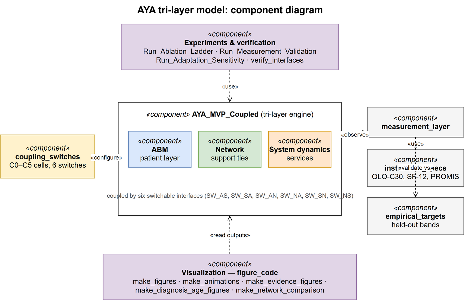
Component diagram: static structure. The AYA_MVP_Coupled engine holds the three layer sub-components and is configured by coupling_switches, driven by the experiment and verification harness, observed through the measurement layer, and read by the visualization code.
  • The tri-layer engine is one component with three internal parts, so the paradigms are coupled in a single integrator rather than chained as separate models
  • coupling_switches configures the engine and the experiment harness drives it, which keeps experiment definitions out of the model code
  • The measurement layer reads instrument specifications and validates against held-out empirical targets, separating observation from dynamics
  • The visualization component (figure_code) depends only on engine outputs, which is why every site figure regenerates from one master script without touching the model
  • Editable source: model_component.drawio / .xml
Stock-and-flow diagram of the system-dynamics services layer
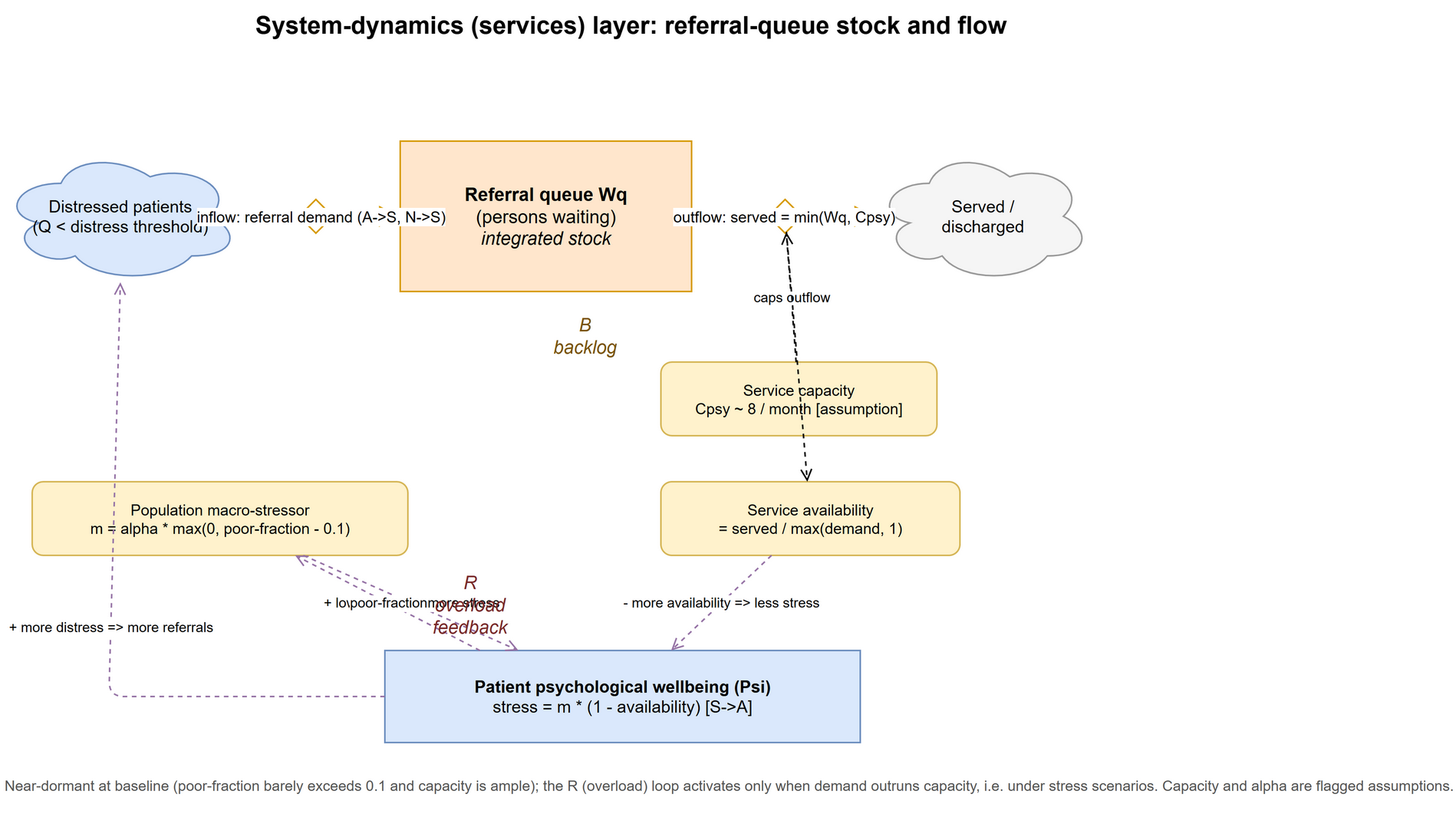
Stock-and-flow diagram: the system-dynamics (services) layer. The services layer is a single integrated stock, the referral queue Wq. Inflow is referral demand (fed by the A→S and N→S interfaces); outflow is the number served, capped by a fixed psychological-service capacity (Cpsy, about 8 per month, a flagged assumption). Service availability (served over demand) and a population macro-stressor feed back to patient psychological wellbeing through the S→A interface.
  • Wq is a true integrated stock: it accumulates unmet demand and drains only as fast as capacity allows, which is what makes this a system-dynamics layer rather than a per-step counter
  • A balancing loop (B) governs the backlog (serving reduces the queue); a reinforcing loop (R) is the overload feedback (a full queue lowers availability, which raises patient stress and distress, which raises demand)
  • At baseline the layer is near-dormant: the poor-fraction barely exceeds the 0.1 macro-stressor threshold and capacity is ample, so the R loop stays latent until a stress or low-capacity scenario activates it
  • Capacity-bounded service is the one channel by which population-level load feeds back to individual wellbeing, matching the single S→A arrow in the sequence diagram
  • Editable source: sd_stock_flow.drawio / .xml

Results

The model was run over 20 simulation seeds and a 24-month horizon. Inference operates at the level of the simulation run rather than the individual agent.

How to read these results:
  • Baseline is the reference a result is compared against (a reduced configuration in the ablation, or the value at month 0 in a trajectory)
  • Emergent is a pattern that arises from the rules of the model itself, rather than a value entered by hand or a target used in fitting
  • Held-out band is a literature target range withheld from calibration, used afterward as an out-of-sample check
  • Population norm is where a healthy general population scores on the same instrument, drawn as a reference line
The headline result is the HRQoL distribution (the violin plot, a shape that shows the full spread): the population stays split into two groups (a higher-faring resilient group and a distinct lower-faring vulnerable group), so the mean recovers yet represents neither group. The animations are the second headline. A fuller plot-by-plot guide is in docs/READING_THE_RESULTS.md.
Ablation ladder
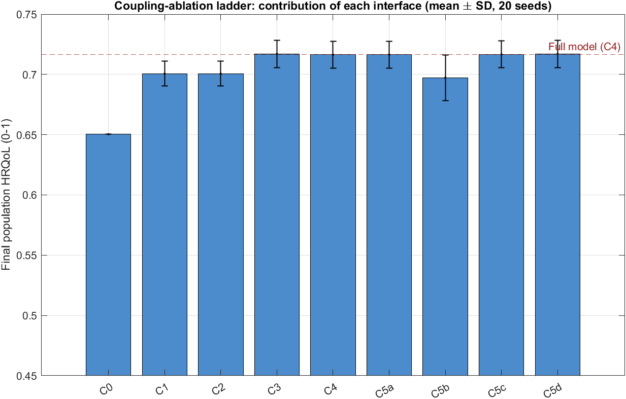
Each interface has a measurable, sign-interpretable effect. Switching couplings on and off shifts population HRQoL in directions the mechanisms predict. The ablation ladder is the core methodological evidence; effect sizes differ sharply across interfaces.
  • Social support (N→A) carries the largest effect: removing it lowers 20-seed mean HRQoL by about 0.020, and adding the network is what raises HRQoL above the agent-only baseline
  • The population-feedback loop (S→A) shifts baseline HRQoL by under 0.002, because the poor-fraction barely exceeds the population-stress threshold; ABM-only and ABM+SD nearly coincide until stress or intervention scenarios activate it
  • Structural feedback (A→N tie dissolution) and the network-population loop move the mean by about 0.001, within seed variation at baseline but mechanistically active during the distress peak
  • The ladder makes the contribution of each layer measurable, including where the baseline effect of a layer is small, which is itself a reported model finding rather than a hidden assumption
HRQoL trajectory
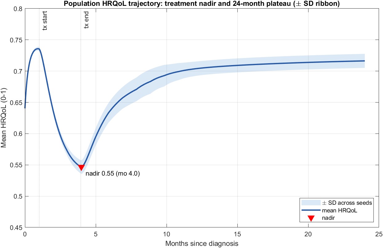
Trajectory shape. HRQoL falls to a low point near month 4, then recovers partially to a 24-month plateau that stays below full health.
  • HRQoL reaches a low point near month 4, then recovers only partially
  • The 24-month plateau stays below full health, matching persistent AYA deficits[2]
  • The coupled dynamics produce the fall-then-recover shape independently; nothing in the model scripts it directly
  • Between-person spread widens during treatment: patients vary in vulnerability and in response to it
Instrument trajectory
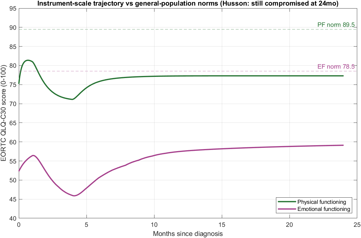
On instrument scales (EORTC QLQ-C30[15]). Physical functioning recovers toward the norm. Emotional functioning stays the deeper, persistent deficit, matching the AYA literature[1, 2]
  • Physical functioning recovers toward the population norm by 24 months
  • Emotional functioning stays the deeper, persistent deficit[1, 2]
  • The physical-over-emotional ordering emerges independently rather than being fitted, which supports behavioral validity
  • Reporting on a real instrument makes the simulation directly comparable to published cohorts
Calibration and validation
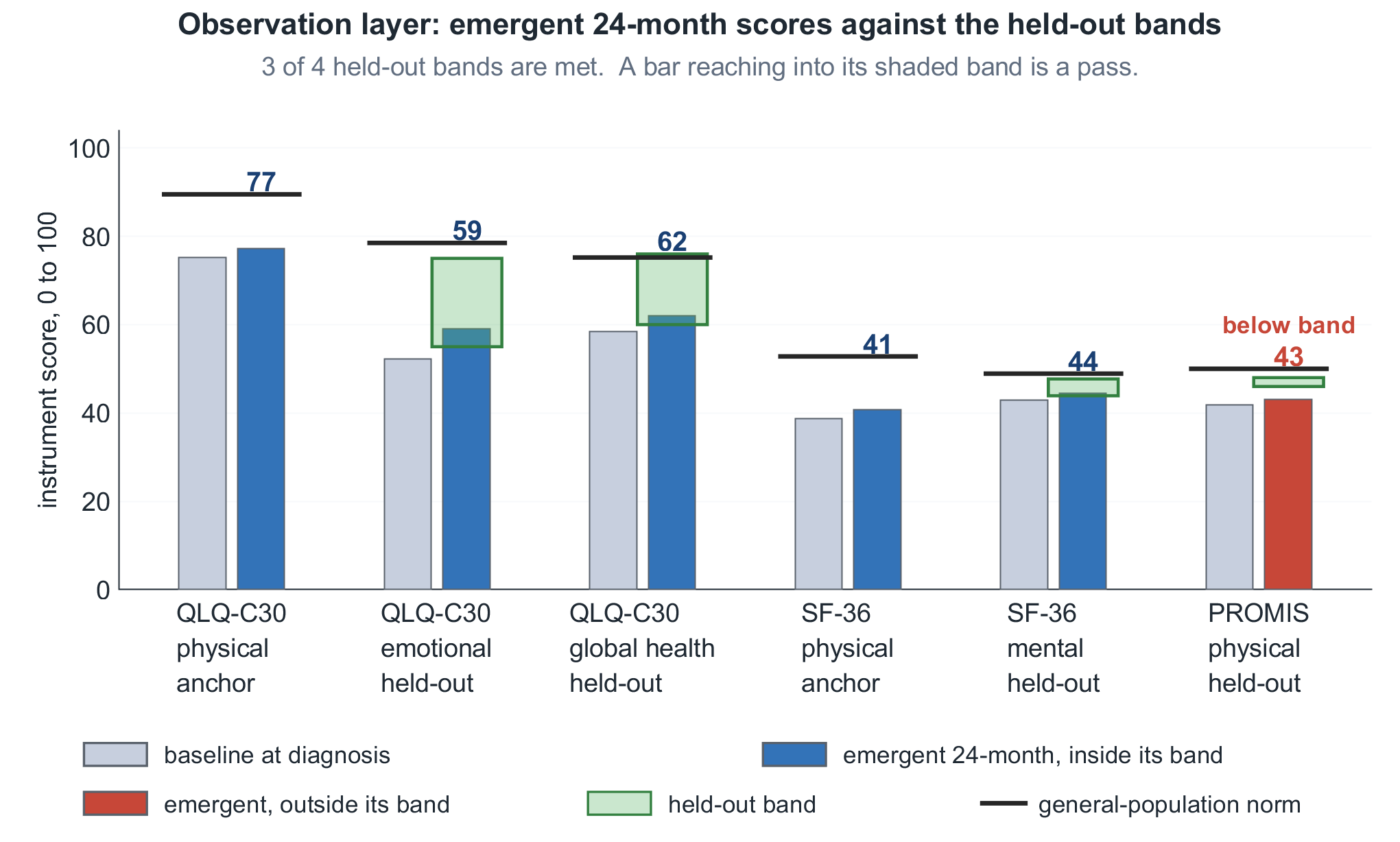
One simulation, several questionnaires. The green bands are literature target ranges set aside from calibration; the emergent 24-month scores land inside them for QLQ-C30, SF-12, and PROMIS[1, 3, 4]
  • All four held-out 24-month instrument targets fall inside literature-derived bands (4/4)
  • One internal (not directly measured) trajectory reconciles the different United States and European questionnaires through the observation layer
  • The targets are excluded from calibration, so agreement functions as a validity check rather than a fit
  • The one early failure (emotional functioning) localized the missing adaptation mechanism
Adaptation sensitivity
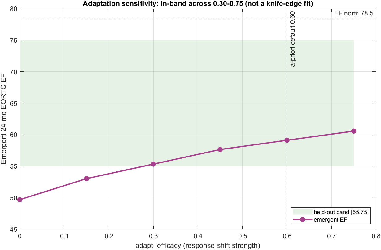
Not a narrowly tuned (i.e. knife-edge) fit. The response-shift adaptation mechanism holds emotional functioning in range across a wide parameter span, with the a-priori default near the middle of that band[10, 11]
  • A response-shift adaptation mechanism brings emotional functioning from 1/4 to 4/4 targets in range[10, 11]
  • The result holds across a wide range of the adaptation strength, so it does not depend on one finely tuned value
  • Theory set the parameters; the bands played no part in tuning them, which keeps the result non-circular
  • Because the mechanism answered a failure, the bands are now development targets; predictive validation needs new data
Stress-scenario ablation of the system-dynamics layer
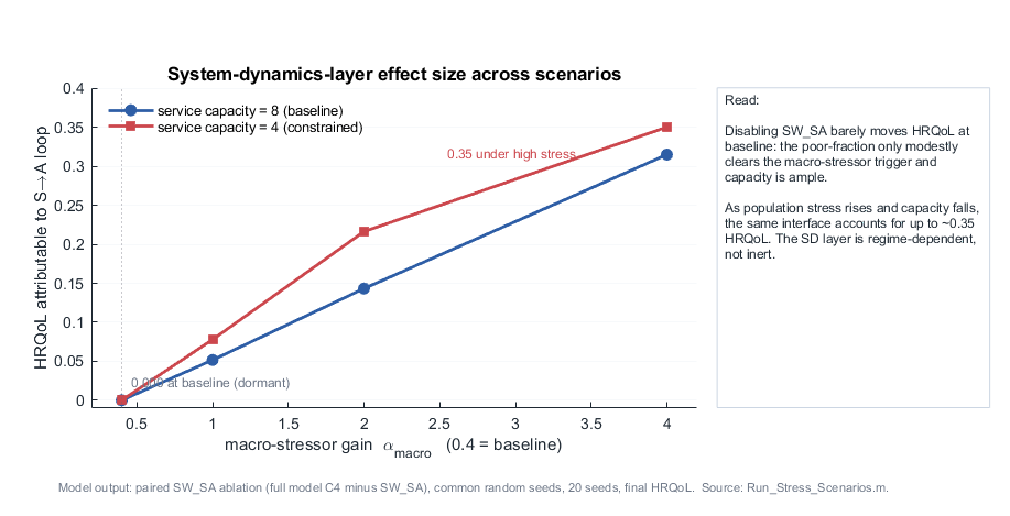
Where the third layer earns inclusion. The ablation ladder shows the system-dynamics population-feedback interface (S→A) is near-dormant at baseline. This experiment varies the population-stress strength and the service capacity and measures the paired S→A ablation effect, so the contribution of the SD layer is shown to depend on the scenario rather than being fixed.
  • At baseline the S→A interface accounts for under 0.001 HRQoL: the population-feedback loop sits genuinely dormant
  • As the population-stress strength rises from 0.4 to 4.0, the same interface accounts for up to about 0.32 HRQoL at baseline capacity
  • Constraining service capacity (8 to 4) amplifies the effect at every stress level, reaching about 0.35 HRQoL, because the referral queue backs up and service availability falls
  • The SD layer is therefore a dormant amplifier that switches on under population stress and scarce capacity, the situations where decision support is most needed
  • Model output: paired SW_SA ablation (full model minus SW_SA), common random seeds, 20 seeds
Individual HRQoL distribution over time
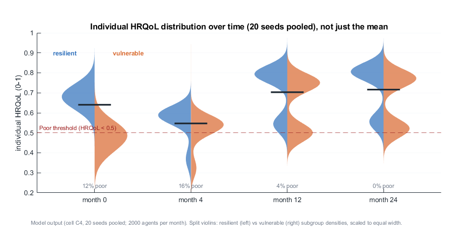
The mean hides the distribution. Per-agent HRQoL pooled over 20 seeds, shown as split violins (resilient left, vulnerable right) at four months. Reporting the full distribution, not just the mean, exposes spread and a persistent low-HRQoL subgroup.
  • The spread is widest at the month-4 low point, when the fraction doing poorly peaks near 15%, so the mean understates how many agents are doing badly mid-treatment
  • A vulnerable subgroup (~20%) forms a distinct lower mode that persists to 24 months, even as the population mean recovers to about 0.72
  • By 24 months the resilient subgroup concentrates near 0.80 while the vulnerable subgroup stays lower and separate, a difference invisible in any mean trajectory
  • Differences in vulnerability and support produce this two-group split independently; no fixed split is imposed after initialization

Headline results

Simulation dynamics (animated)

The animations are rendered directly from a single full-model run (cell C4, all six interfaces on, seed 42) over the 24-month horizon. The first depicts the whole simulation; the rest isolate each layer and the interfaces.

The coupled tri-layer model

Full tri-layer simulation. Four synchronized panels: the support network colored by HRQoL (top left), population mean HRQoL (top right), the system-dynamics referral queue and service availability (bottom left), and the six interface flows for the current month (bottom right). Support (N→A) is active throughout; the referral, service, and tie-dynamics interfaces switch on as treatment-era distress rises.
  • The four panels move together as one coupled system rather than as four independent views
  • The referral queue fills during the treatment-era distress peak and drains as distress subsides
  • Support (N→A) runs throughout; referral, service, and tie interfaces switch on only when distress rises
  • Population HRQoL and the SD queue move in opposition, exposing the population-stress feedback loop

The three layers over time

Agent-based layer. Left: the patient cloud in (physical, psychological) space, colored by HRQoL; psychological wellbeing trails physical through treatment. Right: the Good / Moderate / Poor population fractions shifting over time.
  • The patient cloud stays below the equal-wellbeing diagonal: psychological wellbeing lags physical
  • During treatment the cloud descends, then recovers faster on the physical axis than the psychological
  • Compartments shift toward Moderate and Poor at the low point, then back, but not fully to baseline
  • A vulnerable subgroup (~20%) persists in the Poor compartment, reproducing the two-group AYA pattern[1]
Network layer. The support graph (left): every node is an AYA patient colored by HRQoL, every edge a peer support tie; there are no separate support agents. The right panel tracks mean closure (local clustering), the structural quantity that sets emotional support, alongside mean degree for scale.
  • Closure, not degree, is the quantity the support mechanism keys on, so it is plotted as the primary metric
  • Closure falls over the run (about 0.39 to 0.31) as withdrawal dissolves ties and peer-program formation adds non-clustering ties, so emotional-support capacity declines even as the network stays active
  • Mean degree rises slightly (about 6 to 6.5), moving opposite to closure, which is exactly why mean degree alone is a misleading summary of this network
  • Isolated nodes carry a support penalty: structural position affects individual outcome
Network layer, typed-support extension (exploratory). The same support idea drawn as a single patient spokewheel: the hub is one AYA (color = HRQoL), and each spoke is a typed support tie (family, partner, peer, peer-mentor, clinician, social worker, navigator, digital), with width set by tie strength. Emotional support is the type-weighted sum over active ties, and it drives HRQoL through the same exploratory map used by the static figure[62]
  • Support is specialized by relationship type: family and partner carry the most emotional weight; clinician and navigator carry instrumental weight
  • Ties form over the run (a referral adds a social worker, a peer-support program adds a peer-mentor, a navigator and a partner join) and one peer tie lapses, so the wheel gains and sheds spokes
  • As stronger emotional ties accumulate, type-weighted support rises and HRQoL recovers from the distressed band (about 0.45 to 0.68), with a recovery lag
  • The typed-tie layer is an exploratory extension, not the verified core: tie-type weights are literature-informed estimates and the formation/lapse timeline is illustrative
System-dynamics layer. The referral queue as an integrated stock, with inflow (demand) and outflow (served, bounded by capacity) arrows scaled by magnitude, a service-availability gauge, and the queue level over time.
  • The referral queue is a real integrated stock with explicit inflow and capacity-bounded outflow
  • Demand outruns capacity during the distress peak, so the queue builds and service availability drops
  • As distress subsides, served catches up and the queue drains, restoring availability toward one
  • Capacity-bounded service is the channel by which population load feeds back to individual wellbeing

The six interfaces over time

Coupling between layers. Each directed arrow is one of the six interfaces; the width of each arrow tracks the normalized flow carried that month, and the bars give the same six magnitudes. The order in which the interfaces activate emerges from the coupled dynamics; no fixed schedule drives it.
  • N→A (support) carries flow from the start; the other five interfaces stay dormant until distress appears
  • Referral, service, and tie-dynamics interfaces activate together around the treatment low point
  • Interface magnitudes rise and fall with the distress wave, then quiet as the system recovers

Validation and credibility

With sparse, non-equivalent data, a model like this cannot be validated the way a prediction model is. The argument separates four claims and states which are established and which remain open.

Verification (established). Every interface passes runnable checks, including a no-leak proof that disabling a coupling removes the associated influence[9] DONE
Behavioral validity (partial). The model reproduces several patterns it was not fitted to: baseline deficits, the treatment nadir, durable remission near 78%, and a small intervention effect. The approach is pattern-oriented modeling[7] PARTIAL
Docking against other models (partial). Reduced to the scope of those models, the model reproduces the population-feedback behavior of published system-dynamics HRQoL models[16, 17] and the direction of social-support effects[6], following the model-alignment (docking) method of Axtell et al[8] PARTIAL
Predictive validity (open). No single longitudinal, multidomain, multi-instrument AYA cohort exists to test against. The page states this plainly and gives a roadmap. OPEN

Iterative validation: an informative failure

An early held-out instrument test failed on emotional functioning, passing 1 of 4 targets. The failure was diagnostic: it located a missing response-shift adaptation mechanism[10, 11] Adding that one theory-grounded mechanism brought the test to 4 of 4 across a wide parameter range. Because the mechanism was added in response to the failure, those bands now serve as development targets rather than independent validation. Genuine predictive validation requires new external data.

Objections and responses

"Predictive validation is impossible here, so the work is storytelling."
Validity is purpose-relative[13, 14] Verification, pattern reproduction, and docking are the near-term claim. Predictive validity is scoped as future work with a concrete plan.
"The network is just an ABM term; the SD is just aggregation."
Each layer meets explicit autonomy criteria. The network evolves by independent rules, and the SD layer integrates a real queue stock. The no-leak test shows the contributions are separable[9]
"The parameters are not all sourced."
Every value has a provenance entry. Unsourced values are flagged openly, then handled through sensitivity analysis and an exploratory-modeling stance[12]
"The instruments are not equivalent."
For that reason the model includes an explicit observation layer with measurement error and a calibration/validation split across United States (SF-12, PROMIS) and European (EORTC QLQ-C30) instruments[4]

Full argument, all objections, and references: MODEL_CREDIBILITY_AND_VALIDATION.md.

Comparison to pre-existing models

The exercise below is comparative validation by docking: the novel hybrid is placed alongside pre-existing system-dynamics and agent-based models from the AYA HRQoL literature and reduced to the scope of those models. It is a confidence check, not a change to the model. The model code and every result elsewhere on this page are unchanged; the benchmark only reads the model and compares it.

Five arms were run over the same diagnosis-anchored 24-month horizon, each at a separately documented initialization: an SD-only model (with a common-initialization variant), an ABM-only ablation, an older ABM + static-network hybrid, and the full hybrid. Two literature models are structural comparators only: Q-PRIMA (the published implementation is incomplete and will not run as shipped) and Beaulieu (2022), which is a causal loop diagram rather than a runnable model.

Where this sits in the field. A 2025 PRISMA systematic review of system-dynamics cancer models (Chen et al., Journal of Medical Economics) identified sixteen studies. All are single-paradigm system dynamics, most addressing screening, prevention, or treatment operations at the population level, and produce cases, deaths, quality-adjusted life years, and costs rather than an individual health-related quality-of-life trajectory. None couples an agent-based patient layer, an evolving support network, and a finite-service subsystem, and none tracks HRQoL across survivorship. This architecture addresses that gap. Because those models compute different quantities, they serve as structural comparators only; the graph above does not plot them as additional lines.

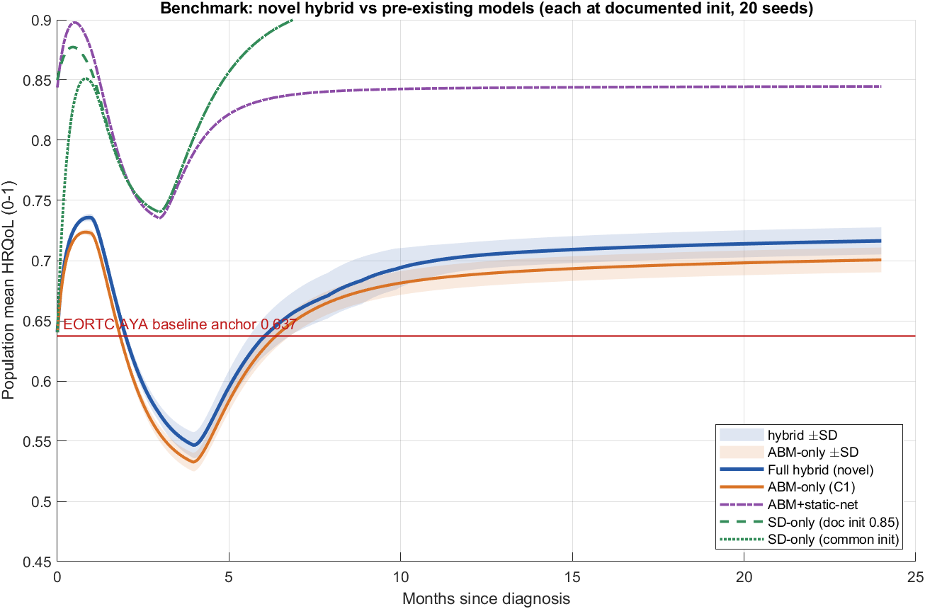
HRQoL trajectories: novel hybrid versus pre-existing models against the empirical anchor
Trajectories against the empirical AYA envelope. The pre-existing SD-only and static-network models sit at 0.83–0.90 for the whole horizon, above the empirical AYA range; the novel hybrid and the corresponding ABM-only ablation show the treatment low point and recover to a below-norm plateau near the matched EORTC baseline (0.6375).
  • Pre-existing designs overshoot because they start high and uniform and lack the two-group initialization and the identity and financial penalties
  • The SD-only overshoot persists even when it is started at the baseline value of the hybrid, so the dynamics themselves produce it, independent of the initial condition
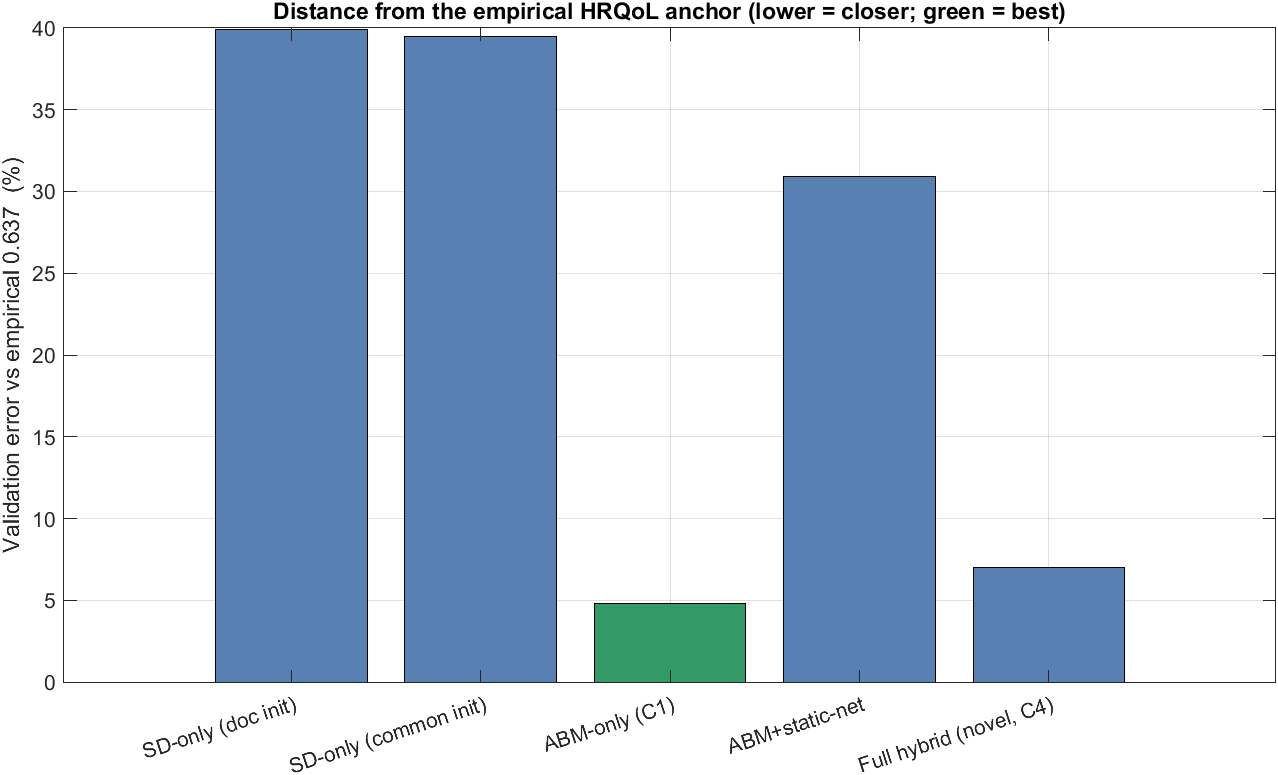
Distance from the empirical HRQoL anchor by model
Distance from the empirical anchor. Lower is closer. The novel model family is 5–7% from the anchor; the pre-existing models are 31–40%.
ModelTime-avg HRQoLDistance from empirical anchor 0.6375
SD-only (documented init 0.85)0.89239.9%
SD-only (common init)0.88939.5%
ABM + static-network0.83530.9%
ABM-only (C1)0.6684.8%
Full hybrid (novel, C4)0.6837.2%
Support network over 24 months (benchmark run). The evolving adjacency captured by the benchmark, nodes colored by HRQoL. The full N×N adjacency at each month is saved to benchmark_comparison/mat/adjacency_over_time.mat.
Read with care. The docking supports the model family over the pre-existing designs. It does not establish the full hybrid over the ABM-only ablation on this single mean-fit metric (ABM-only 4.8% versus full 7.2%); the added value of the full model stays with the ablation and distributional evidence in the Results and Validation sections. The empirical anchor is a construct-matched EORTC value that remains provenance-flagged, so the percentage column functions as a relative yardstick rather than a settled fit. The conclusion does not hinge on the exact anchor: the pre-existing models spend the whole horizon above the empirical AYA envelope while the novel family stays within it.

Reproducible as a standalone folder: benchmark_comparison/ with run_benchmark(20). Details in benchmark_comparison/README.md, the anchor trace in ANCHOR_RECONCILIATION.md, and the structural comparison in tables/structural_docking.csv.

Future work

The model is a verified prototype with an open predictive-validation claim and several scoped limitations. The priorities below would close those gaps, ordered from the most decisive (external validation) to incremental refinements.

Predictive validation

Diagnosis and age

Model structure and scope

Verification, docking, and uncertainty

Collaboration

A model of this scope needs data and domain expertise that no single project holds. The project seeks:

Studies traced, and the specific data requested

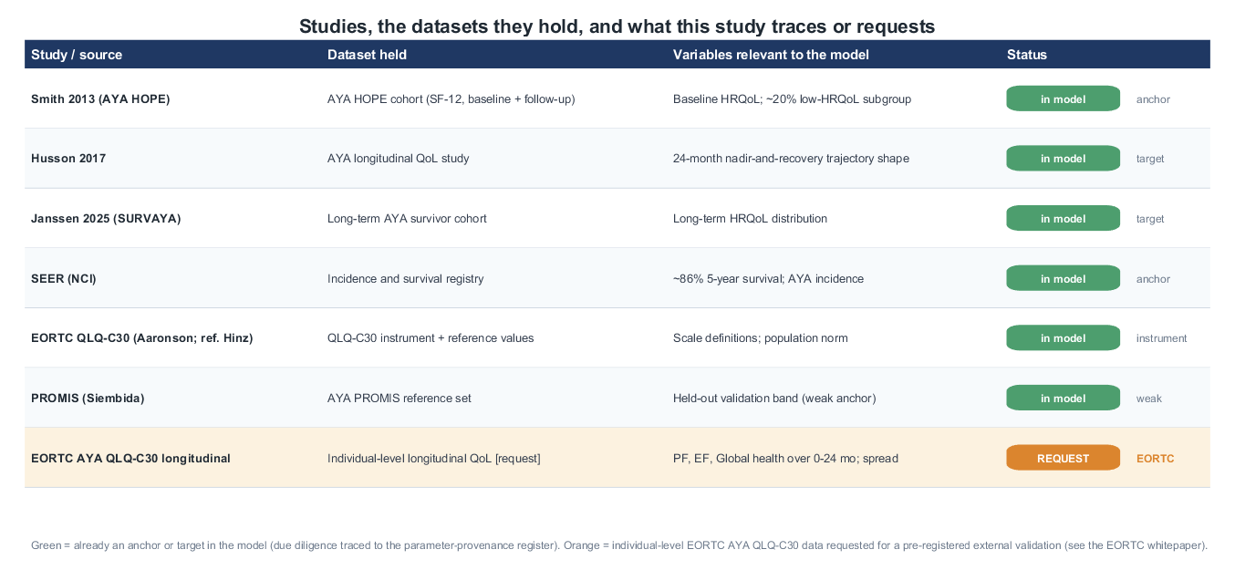
The figure traces the studies and datasets this project already relies on (due diligence, each tied to the parameter-provenance register) and identifies the one dataset requested to close the open validation question: individual-level EORTC QLQ-C30 longitudinal data in AYA patients. An EORTC data-request has been placed to compare individual-level, longitudinal quality-of-life data against the tri-layer model.

Studies, the datasets they hold, and what is already in the model versus requested from EORTC
Studies, datasets, and the EORTC request. Green rows are anchors or targets in the model; the orange row is the individual-level EORTC AYA QLQ-C30 dataset requested for external validation.
  • Each in-model source is traced to a specific role: an initialization anchor, a validation target, an instrument, or a population norm
  • Requested EORTC data is read on the same QLQ-C30 scales the model already emits, so the external test needs no additional crosswalk assumptions
  • Usage is confirmatory: the model is locked, the compared quantities and acceptance criteria are registered before the data are seen

Questions? Contact: jblochb2@jhu.edu

References

  1. A. W. Smith et al., "Health-related quality of life of adolescent and young adult patients with cancer in the United States: the Adolescent and Young Adult Health Outcomes and Patient Experience study," Journal of Clinical Oncology, vol. 31, no. 17, pp. 2136–2145, 2013
  2. O. Husson et al., "Health-related quality of life in adolescent and young adult patients with cancer: a longitudinal study," Journal of Clinical Oncology, vol. 35, no. 6, pp. 652–659, 2017
  3. Janssen et al., "Health-related quality of life of long-term adolescent and young adult cancer survivors: the SURVAYA study," Journal of Cancer Survivorship, 2025
  4. A. Hinz et al., "European reference values for the quality of life questionnaire EORTC QLQ-C30," Acta Oncologica, vol. 53, no. 7, pp. 958–965, 2014
  5. Surveillance, Epidemiology, and End Results (SEER) Program, National Cancer Institute, "Cancer stat facts: adolescent and young adult (AYA) cancers (ages 15–39)," https://seer.cancer.gov/ (5-year relative survival)
  6. M. Pinquart and P. R. Duberstein, "Associations of social networks with cancer mortality: a meta-analysis," Critical Reviews in Oncology/Hematology, vol. 75, no. 2, pp. 122–137, 2010
  7. V. Grimm et al., "Pattern-oriented modeling of agent-based complex systems: lessons from ecology," Science, vol. 310, no. 5750, pp. 987–991, 2005
  8. R. Axtell, R. Axelrod, J. M. Epstein, and M. D. Cohen, "Aligning simulation models: a case study and results," Computational and Mathematical Organization Theory, vol. 1, no. 2, pp. 123–141, 1996
  9. R. G. Sargent, "Verification and validation of simulation models," Journal of Simulation, vol. 7, no. 1, pp. 12–24, 2013
  10. M. A. G. Sprangers and C. E. Schwartz, "Integrating response shift into health-related quality of life research: a theoretical model," Social Science & Medicine, vol. 48, no. 11, pp. 1507–1515, 1999
  11. K. M. Bellizzi et al., "Positive and negative psychosocial impact of being diagnosed with cancer as an adolescent or young adult," Cancer, vol. 118, no. 20, pp. 5155–5162, 2012
  12. S. Bankes, "Exploratory modeling for policy analysis," Operations Research, vol. 41, no. 3, pp. 435–449, 1993
  13. Y. Barlas, "Formal aspects of model validity and validation in system dynamics," System Dynamics Review, vol. 12, no. 3, pp. 183–210, 1996
  14. G. E. P. Box, "Science and statistics," Journal of the American Statistical Association, vol. 71, no. 356, pp. 791–799, 1976
  15. N. K. Aaronson, S. Ahmedzai, B. Bergman, et al., "The European Organization for Research and Treatment of Cancer QLQ-C30: a quality-of-life instrument for use in international clinical trials in oncology," Journal of the National Cancer Institute, vol. 85, no. 5, pp. 365–376, 1993
  16. Z. Hasgul, A. Spanjaart, S. Javed, A. Akhavan, M. J. Kersten, and M. S. Jalali, "Health-related quality of life dynamics: modeling insights from immunotherapy," Quality of Life Research, vol. 34, no. 1, pp. 273–286, 2025
  17. E. Beaulieu, A. Spanjaart, A. Roes, B. Rachet, S. Dalle, M. J. Kersten, D. Maucort-Boulch, and M. S. Jalali, "Health-related quality of life in cancer immunotherapy: a systematic perspective, using causal loop diagrams," Quality of Life Research, vol. 31, pp. 2357–2366, 2022
  18. E. S. Kenzie, M. Seater, W. Wakeland, G. D. Coronado, and M. M. Davis, "System dynamics modeling for cancer prevention and control: a systematic review," PLOS ONE, vol. 18, no. 12, art. e0294912, 2023
  19. A. Gjerloev, S. Crowe, C. Pagel, Y. Jani, and L. Grieco, "A systematic review of simulation methods applied to cancer care services," Health Systems, vol. 13, no. 4, pp. 274–294, 2024

Data sources and model-building bibliography

References grounding the parameters, instruments, methodology, and validation of the model, drawn from the project literature review and the source papers used to build the model.

AYA cancer HRQoL: field, outcomes, and policy

HRQoL measurement instruments and care guidelines

Social, psychological, and survivorship mechanisms

System-dynamics and hybrid simulation of cancer and health

Agent-based and computational oncology

Simulation verification and validation methodology

Network science and social contagion

Parameter-provenance sources (verified)

Public datasets